LLMs from First Principles

You know what AI is, right? But can you also explain how an LLM actually works?

I got into machine learning before GPT-3 came out and I use LLMs almost every day for coding, research and all my side projects. I’m more on the product side though, so I only touched ML a few times.

A few days ago a tweet about hiring asked what the most advanced technical concept is that you can actually explain. I tried to explain LLMs in my head and got stuck pretty fast. I could say “transformer” and “attention” but I had no clue how attention or the training actually work.

So after watching GreenCode build his own LLM, I went on a quest to build my own GPT using only NumPy. I trained it on TinyStories, a dataset of short stories written with the vocabulary of a 3 to 4 year old. It’s small and simple, which is perfect, because even models with fewer than 10 million parameters can learn to write fluent little stories with it. The code is on GitHub if you want to have a look -> joelGPT.

What an LLM is

A Large Language Model is a function that takes some text and returns a probability for every possible next piece of text. ChatGPT is that function called in a loop. It predicts one token, appends it and predicts again, just on an extremely large scale.

Under the hood that function is a lot of multiplications with adjustable numbers called weights (or parameters), which start out random. Training means finding values for them that make good predictions and usable text.

GPT stands for Generative Pre-trained Transformer.

• Generative because it generates text, one token at a time.
• Pre-trained because it first learns from a huge pile of text by doing nothing but predicting the next token. Behaviour like answering questions gets added later with fine-tuning.
• Transformer because that is the architecture, introduced in Attention Is All You Need in 2017. GPTs use only the “decoder” half of it.

This picture shows everything an LLM is made of and I’ll go through it step by step.

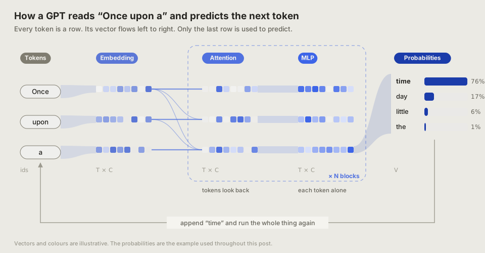
The small labels are the shapes of the data. T is the number of tokens, C is how many numbers we use per token and V is the number of different tokens the model knows. MLP (Multi Layer Perceptron) is the feed-forward network.

If you want to play with a live version of this picture, try Transformer Explainer by the Polo Club of Data Science at Georgia Tech. It runs a real GPT-2 in your browser, you can type your own text and watch every step. It was a big inspiration for the images in this post.

Load Transformer Explainer Downloads GPT-2 (about 600 MB) into your browser, so it only loads on click.

1. Tokens: Turning text into numbers

Computers can’t do math on words, so the first step is to cut text into pieces called tokens and give each piece an id.

You could use single characters (few different pieces, but very long sequences) or whole words (short sequences, but a gigantic list of words and no way to handle a word you have never seen). GPT uses something in between called byte pair encoding (BPE, Sennrich et al.). It was borrowed from data compression so that rare words can still be built out of smaller known pieces a bit like using Lego bricks to build up any word that you can encounter.

The algorithm is almost stupidly simple. Start with single characters, count which pair of neighbours shows up most often, glue it into a new token and repeat.

After a few thousand merges common words like “the” are a single token, while rare words get split into chunks. The list of all tokens is called the vocabulary. My hand-written model skips BPE and uses 91 single characters, the bigger version further down uses 4,096 BPE tokens and GPT-2 has 50,257.

2. Embeddings: Giving every token a meaning

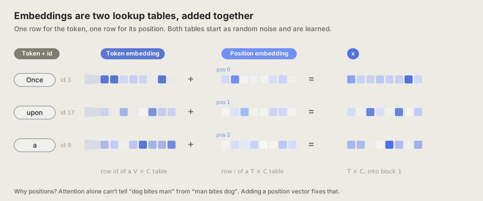
A token id like 17 is just a name and the number itself says nothing about the word and its meaning. Token 17 isn’t more similar to token 18 than to token 900. To give the model something it can calculate with, we turn every token into a list of numbers (a vector) to show their meaning is too each other in a multi dimensional space.

We do that with a big table that has one row of numbers for every token in the vocabulary and to get a token’s vector we just look up its row.

# one row per token
token_table = np.random.randn(vocab_size, vector_size) * 0.02

# one vector per token
vectors = token_table[token_ids]

The table starts random and every number in it gets tuned during training. Tokens that are used in similar ways slowly drift close together and others drift apart. Even directions in this space start to mean something, like the step from “mom” to “dad” or from “happy” to “sad”.

Positions

The model also needs to know where each token is, because attention (next section) has no idea about order. It sees the tokens like a bag of words, so “dog bites man” and “man bites dog” would look identical. That’s why we add a second learned table with one row per position and add it on top.

# one row per position
position_table = np.random.randn(context_length, vector_size) * 0.02
vectors = token_table[token_ids] + position_table[:len(token_ids)]

Now the vector for “dog” at position 0 is different from “dog” at position 2. GPT-2 does exactly this, newer models use fancier tricks for positions.

3. Attention: Letting tokens talk to each other

Attention is the heart of the whole thing. After the embedding step, the vector for a word knows nothing about its neighbours. Take the word “mole” (3Blue1Brown’s example).

• American shrew mole
• one mole of carbon dioxide
• take a biopsy of the mole

It is the same token and the same vector, but it has three completely different meanings. Attention is the step where every token looks at the tokens before it and pulls in whatever is relevant.

To do that, each token creates three new vectors by multiplying its vector with three learned matrices.

• Query. “What am I looking for?” -> noun might ask “is there an adjective in front of me?”
• Key. “What do I contain?” -> adjective might answer “I’m an adjective”.
• Value. “If you find me relevant, here is the information I’ll hand you.”

This took me a while to get until I realized that the model doesn’t know what an adjective or a noun is. Meaning and grammatical rules only show up because words appear next to each other or in similar sentences during training when trying to predict the next token.

We measure a match with the dot product. You multiply two vectors number by number and add everything up. If they point in the same direction the result is big, if they point in opposite directions it’s negative.

A matrix multiplication is many dot products at once. Every row on the left gets multiplied with every column on the right. In NumPy that is the @ sign and it is almost all an LLM ever computes.

We then use softmax to turn scores into percentages. It makes every score positive with e^score and then divides by the total, so everything adds up to 100%.

Bigger scores therefore get a bigger share and we can calculate it using this formula:

$$\text{Attention}(Q, K, V) = \text{softmax}\left(\frac{QK^\top}{\sqrt{d}}\right)V$$

Read it from the inside out.

1. QKᵀ gives a score for every pair of tokens, every query against every key
2. Divide by √d, where d is the length of the key vectors. Longer vectors give bigger scores and huge scores make softmax put almost 100% on one token, which stops learning. Dividing keeps the scores in a normal range
3. Hide the future. A token should only look at tokens before it. During training the model predicts every next token at the same time, so if “a” could see “time” it would just copy the answer. We set those scores to −∞, which softmax turns into 0%
4. Softmax turns each row of scores into percentages
5. Multiply with V. Each token’s new vector is a mix of the values it pays attention to

def softmax(scores):
    # subtracting the max avoids huge numbers
    exp_scores = np.exp(scores - scores.max(axis=-1, keepdims=True))
    # every row adds up to 1
    return exp_scores / exp_scores.sum(axis=-1, keepdims=True)

def attention(vectors, query_weights, key_weights, value_weights):
    queries = vectors @ query_weights
    keys = vectors @ key_weights
    values = vectors @ value_weights
    # every token against every token
    scores = queries @ keys.T / np.sqrt(keys.shape[1])
    # hide the future: everything above the diagonal
    is_future = np.triu(np.ones(scores.shape), k=1) == 1
    scores[is_future] = -np.inf
    # mix the values
    return softmax(scores) @ values

Multi-head attention

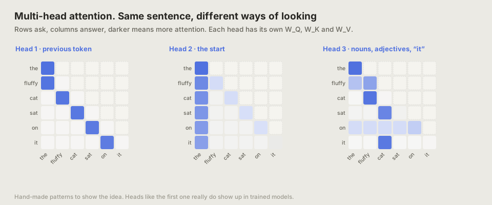
One set of query, key and value can only learn one kind of “looking”. One head might connect adjectives to nouns, another might figure out what “it” refers to. So the model runs several smaller heads side by side, each with its own three matrices. Their outputs get glued together and mixed with one more matrix. Because each head is smaller, the total work is about the same as one big head.

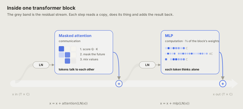
4. Residual connections and LayerNorm

Residual connections

After attention we don’t replace a token’s vector with the result, but add the result on top of it.

vectors = vectors + attention(layernorm(vectors))
vectors = vectors + feed_forward(layernorm(vectors))

This way each step only has to learn a small change (“add a bit of adjective info to this noun”) instead of rebuilding the whole vector and nothing gets lost because the original token is still in there after many blocks. Anthropic’s transformer circuits paper calls this the “residual stream”, one stream of vectors flowing through the model that every step reads from and adds to.

LayerNorm

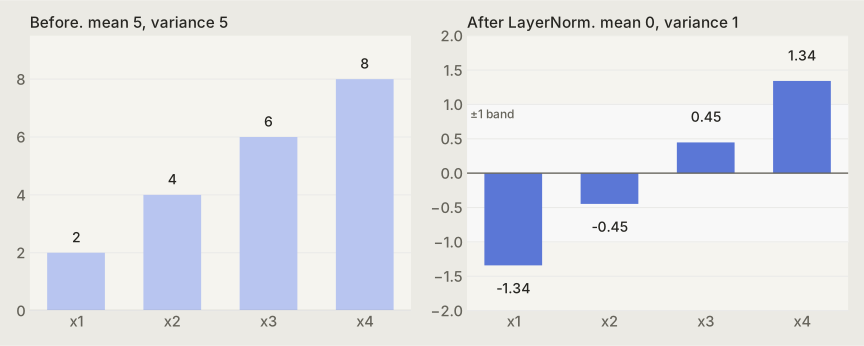
Every block multiplies the vectors with more matrices. Multiply by numbers a bit bigger than 1 again and again and the values explode, a bit smaller than 1 and they vanish. LayerNorm prevents that by resetting every vector to a normal size before each step (the pictures call it LN).

It takes each token’s vector, subtracts its average and divides by its spread (the standard deviation). The result always has an average of 0 and a spread of 1. Then it gets multiplied by a learned scale and shifted by a learned offset, so the model can still adjust it.

def layernorm(vectors, scale, shift):
    mean = vectors.mean(axis=-1, keepdims=True)
    std = vectors.std(axis=-1, keepdims=True)
    return scale * (vectors - mean) / (std + 1e-5) + shift

The original transformer applied LayerNorm after each step. GPT-2 moved it to the start of each step because that makes training much more stable.

5. The feed-forward network

If you have not lived under a rock, you have probably heard about neural networks. Layers of “neurons”, where each neuron multiplies its inputs with weights, adds them up and pushes the result through an activation function.

In a transformer it’s called the feed-forward network or MLP (multi-layer perceptron) in the pictures and most code. In this case we just calculate two matrices with an activation in between and apply it to every token on its own.

def feed_forward(vectors, up_weights, down_weights):
    # make the vector 4x longer
    before_relu = vectors @ up_weights
    hidden = np.maximum(0, before_relu)
    # back to the original size
    return hidden @ down_weights

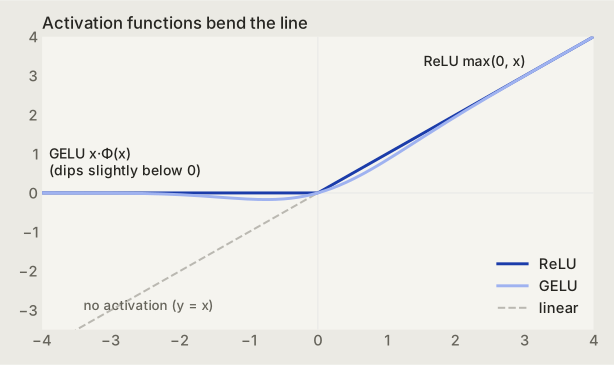
Why the activation function matters

Without an activation, two matrix multiplications in a row are just one matrix multiplication. You could stack a hundred layers and still only ever draw straight lines. The activation is used to bend these functions and is the reason why neural networks can build highly complex functions. My model uses ReLU, which sets every negative number to 0, while GPT-2 uses GELU, a smoother version of it.

So what does it do?

If we view attention as the communication step, the feed-forward network is the thinking step, where each token processes what it collected on its own. Two thirds of each block’s weights sit here and research suggests these layers work like a memory (Geva et al.). The first matrix detects patterns in the input, the second pushes up the tokens that usually follow that pattern. I highly recommend 3Blue1Brown’s video on this.

6. From vectors to a prediction

After the last block, each token still holds a vector. The output layer is one more matrix that turns the vector of the last token into one score for every token in the vocabulary. These raw scores are called logits.

The same softmax as in attention turns them into probabilities. These are made-up scores for what comes after “Once upon a”.

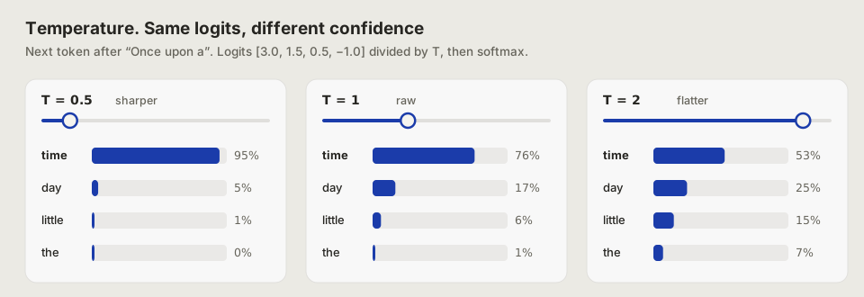
Before the softmax we can divide all scores by a number called temperature. A low temperature makes the model more confident and more boring, a high temperature gives the weird words a chance. That slider in every AI playground is literally dividing by a number before the softmax.

7. How it learns

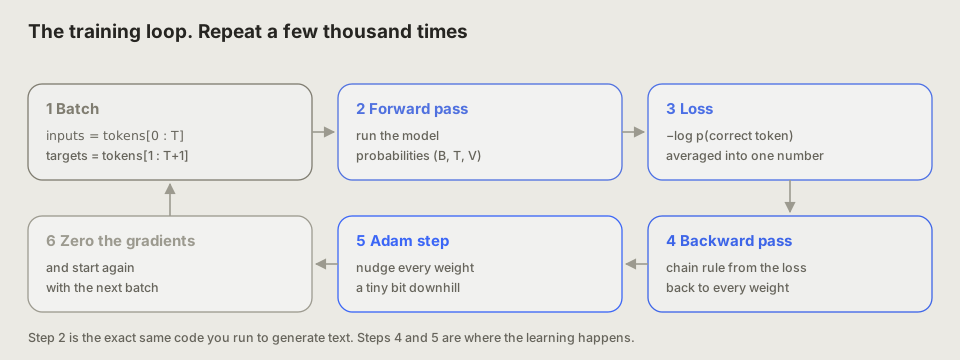
Everything so far is the forward pass and with random weights it outputs garbage. Learning means nudging every single weight (the tables, all the attention matrices, the feed-forward networks and the output layer) so the garbage gets a little less garbage. One training step looks like this.

The training data is free

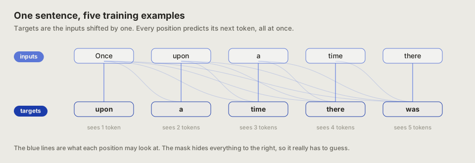
Usually in machine learning someone has to label the data, but in LLMs you don’t as by using any text, the answer is always just the next token. The inputs are the tokens and the targets are the same tokens shifted by one (predicting which token comes next). So one chunk of 256 tokens gives you 256 training examples for free.

Loss: how wrong are we?

The loss is the metric that says how bad the model’s guess was. We look at the probability the model gave the right next token.

$$\text{loss} = -\log(p_{\text{correct}})$$

The log turns probabilities close to 100% into a number close to 0 and probabilities close to 0% into a big number. So the lower the loss, the better. We average it over every position to get one number.

This is called cross-entropy, which sounds fancy but just means how surprised the model was by the right answer.

Backpropagation: how a model learns

Learning means making the loss as small as possible. To do that, we want to know one thing for every weight. If I nudge it up a tiny bit, does the loss go up or down and by how much? That number is called the gradient.

The naive way is to nudge each weight and run the model again. With millions of weights that’s millions of runs for a single training step. Backpropagation gets all gradients in one pass. We start at the loss and work our way backwards through the model, using the chain rule from school: outer derivative times inner derivative, again and again, layer by layer.

A tiny example. Say y = 3w and loss = y². Nudging w changes y 3 times as much and nudging y changes the loss by 2y. So the gradient of w is 3 · 2y. With w = 1 that’s 3 · 6 = 18. An LLM is the same thing, just with millions of these links chained together.

The very first step backwards is simple. For each score, the gradient is what the model said minus what it should have said. I won’t derive it here, it falls out when you take the derivative of softmax and the log together.

$$\text{gradient} = p - y$$

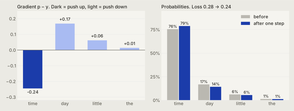
For “Once upon a” the model said [0.76, 0.17, 0.06, 0.01] and the truth is [1, 0, 0, 0], because “time” was right. So the gradient is [−0.24, 0.17, 0.06, 0.01]. Negative means push this score up, positive means push it down.

probabilities = softmax(scores)
positions = range(len(targets))
loss = -np.log(probabilities[positions, targets]).mean()

# what it said minus what it should have said
grad_scores = probabilities.copy()
grad_scores[positions, targets] -= 1
# because we took the average
grad_scores /= len(targets)

From there you push this gradient back through every layer, so each layer you write needs a forward and a backward function. This is where I spent most of my time.

The good news is that almost every backward step follows one rule. For output = inputs @ weights, the gradient for the weights is inputs.T @ grad_output and the gradient you hand to the layer before is grad_output @ weights.T. Everything else is the derivative of whatever sits in between. Here is the backward pass of the feed-forward network from my model.

def feed_forward_backward(grad_output, vectors, before_relu, up_weights, down_weights):
    hidden = np.maximum(0, before_relu)
    grad_down_weights = hidden.T @ grad_output
    # ReLU only lets the gradient through where it was active
    grad_before_relu = (grad_output @ down_weights.T) * (before_relu > 0)
    grad_up_weights = vectors.T @ grad_before_relu
    # hand the gradient to the layer before
    grad_vectors = grad_before_relu @ up_weights.T
    return grad_vectors, grad_up_weights, grad_down_weights

Attention and LayerNorm work the same way, just with more steps. You can read all of them in joel_gpt.py. If you want to see backprop built from zero, Karpathy’s micrograd video is the best two hours you can spend. If you need more intuition on the math and logic behind backprop, I highly recommend this explainer video

Adam, the optimizer

Like the slope of a function from high school, the gradient tells us how steeply the loss goes up or down when we nudge a weight. If it’s positive, making the weight bigger makes the loss worse, so we make it smaller. If it’s negative, we make it bigger.

weight = weight - learning_rate * gradient

This is called gradient descent and the learning rate is the step size. If it’s too big you jump over the best spot, if it’s too small training takes forever. It works, but it has two problems.

Problem 1. It zig-zags. Picture the loss as a long narrow valley. The gradient mostly points at the steep walls, so you bounce side to side instead of walking along the bottom. The fix, called momentum, is to follow the average of the last few gradients, so the bounces cancel out and the real direction adds up.

Problem 2. One step size doesn’t fit all. Some weights get gradients around 100, others around 0.01. The fix is to divide each gradient by its usual size, so every weight moves about the same amount.

Both fixes together are called Adam (Kingma & Ba).

# fix 1: average direction
average = 0.9 * average + 0.1 * gradient
# fix 2: usual size
size = 0.999 * size + 0.001 * gradient**2
weight = weight - learning_rate * average / (np.sqrt(size) + 1e-8)

Real Adam adds one small correction because both averages start at zero, but this is the whole idea.

8. Generating text

After training is done the fun part starts, because generating text is just the forward pass in a loop.

def generate(token_ids, n_new_tokens, temperature=0.8):
    for _ in range(n_new_tokens):
        # the model only fits so many tokens
        scores = model(token_ids[-context_length:])
        # prediction for the next token
        probabilities = softmax(scores[-1] / temperature)
        next_id = np.random.choice(len(probabilities), p=probabilities)
        token_ids = np.append(token_ids, next_id)
    return token_ids

Why pick randomly instead of always taking the most likely token? Always taking the top token makes the text repetitive and it easily gets stuck in loops, while picking by probability keeps it varied.

That’s ChatGPT. Well, minus a few hundred billion parameters, a lot of fine-tuning and some very clever engineering to make it fast. But the loop is the same :)

What my model learned

My NumPy model

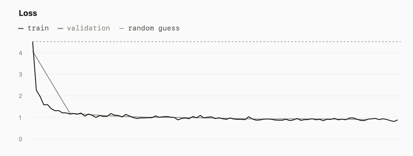
The model I wrote by hand, joel_gpt.py, is pure NumPy. It has 4 blocks, 4 attention heads, 128 numbers per token and reads single characters, about 0.8 million weights in total. It trains in about 30 minutes on my laptop and ends at a loss of 0.88 per character.

It wrote these two stories, both starting from “Once upon a time”.

Once upon a time, in a small house, there lived a tall girl named Sue. Sue wanted to help her. Sue loved to go home back inside, time to go home in you and they always shared the meess.

Once upon a time, there was a little girl who lived in a small house. One day, she found a lestage snack near the enormous that had a girl that when you need it. One day, the milver took the cride back to his room and gave him the bird.
"How like that chill with them." They were very happy.

Not bad for something that only ever sees one letter at a time. It learned to spell most words and even uses quotes for dialogue. But it also makes up words like “meess” and “milver” and most sentences lose the plot halfway through.

The bigger model

To see how far the same idea goes, I had AI write a bigger PyTorch version, ai_gpt.py, based on recent research on training small models fast. It is the same architecture with newer parts: rotations for positions (RoPE) instead of a position table, RMSNorm instead of LayerNorm, a gated feed-forward network (SwiGLU) and the Muon optimizer next to Adam. It has 8 blocks, 6 attention heads, 384 numbers per token, a vocabulary of 4,096 BPE tokens and about 16 million weights and looks at up to 256 tokens (about 1,000 characters) at once. Training took about 7 hours on a MacBook GPU.

The samples below come from an earlier version of ai_gpt.py. The current file adds a few more tricks that I haven’t trained yet.

Step 0 (untrained, loss 8.77)

once upon a time time time time time time time ... lake lake lake lake lake lake lake ...

With random weights, a loss of 8.77 means the right token got about 0.02%. That is slightly worse than guessing evenly between 4,096 tokens, which gives a loss of 8.32.

Step 1,000 (loss 1.76, about 14 minutes of training)

once upon a time, there was a little girl named Tim. Tim had a pet fish named Bob. They were best friends. They talked and laughed together. Tim said, "I hate the sea. It's boring."
One day, a rare fish swam up to Bob and said, "Me too! Let's all fly together!" Sam was happy and said, "Yes, let's go!" They played and had fun.
Then, something unexpected happened. A big fish jumped out and scared them. The fish said, "I don't like the spicy fish. I won't give us a spicy." Tim was surprised but als

The grammar is already there but the logic isn’t: Tim is a girl and Sam shows up out of nowhere.

After training (step 34,146, loss 1.21)

once upon a time, there was a little boy named Tim. Tim loved to play in the sand. One day, he went to the beach with his mom and dad.
At the beach, Tim saw a big sand castle. He wanted to join the kids and make a big sand cake. Tim found a big, tight hug from his mom and dad. He hugged the tight hug and smiled.
Tim went into the sand castle and played with the other kids. They all had fun in the tight sand castle. When it was time to go home, Tim waved goodbye to his new friends. They all had a

A loss of 1.21 means that on a typical token the model gives the right answer about 30% (e^−1.21), out of 4,096 options and the story stays on one topic from start to end.

Here is one more story from the finished model, fresh from my laptop.

Once upon a time, there was a little boy named Tim. Tim loved to draw with his pencil. One day, he went outside to draw a big sun on the ground. He was very happy.
Tim saw a big tree and thought it would be fun to draw it with his pencil. He took out his pencil and started to draw the sun. But, he was careless and did not look where he was going.
As Tim drew the sun, he slipped and fell. Tim's pencil went flying and broke into many pieces. Tim was sad and knew he should have been more careful. The moral of the story is to always look where you are going and be careful when playing outside.

It even ends with a moral, like many stories in TinyStories do. Every word is real and the story has an actual plot: Tim gets careless, breaks his pencil and learns from it. Compared to my NumPy model above, the idea is the same. This model is just 19 times bigger, sees 15 times more text at once and trained for 7 hours instead of 30 minutes.

What I got wrong

Writing the first draft of this post was humbling, so here is what I got wrong and where AI corrected me.

• Embeddings aren’t counted from word pairs, they start random and are learned
• A token only looks at the tokens before it, never after
• Learning happens in the backward pass, not the forward pass
• The feed-forward network works on the vector size, the vocabulary only shows up at the very end
• LayerNorm doesn’t squash values into −1 to +1, it resets every vector to an average of 0 and a spread of 1
• Multiple heads aren’t for speed, each one learns a different relationship
• Transformer blocks run one after another, only tokens and batches run in parallel

From my toy to GPT-3

My first instinct was that GPT-3 must use completely different concepts, but it is more or less the same. The GPT-3 paper says they used the same model and architecture as GPT-2, with one exception: some layers use a sparse attention pattern so long texts get cheaper.

What changes is scale. GPT-3 has 96 blocks, 96 heads and 12,288 numbers per token. Then there is a mountain of engineering to train that on thousands of GPUs, plus fine-tuning and RLHF to turn a story completer into an assistant. But if you understand the 60 lines in Jay Mody’s picoGPT, you understand the core of all of it.

Resources that helped

Writing it in pure Python will take a while and you will need help from peers, Google or AI. My one tip is to use AI as a tutor, not as an autocomplete and to ask it for hints instead of solutions. When you get stuck on a concept, watch a video on exactly that concept.

Videos

• Let’s build GPT from scratch by Andrej Karpathy. The end-to-end walkthrough.
• Building micrograd by Karpathy. Backprop from zero.
• Let’s build the GPT tokenizer by Karpathy. Everything about BPE.
• Transformers, the tech behind LLMs by 3Blue1Brown
• Attention in transformers, step by step by 3Blue1Brown
• How might LLMs store facts by 3Blue1Brown. The feed-forward chapter.
• Attention for neural networks by StatQuest. The math, slowly.
• This video on backpropagation

Interactive

• Transformer Explainer by the Polo Club of Data Science at Georgia Tech (paper). Runs GPT-2 in your browser and lets you play with temperature.
• LLM Visualization by Brendan Bycroft. A 3D walk through every single matrix multiplication.

Reading

• GPT in 60 lines of NumPy by Jay Mody
• Build a Large Language Model (From Scratch) by Sebastian Raschka

Papers (more readable than you’d think)

• Attention Is All You Need, the transformer
• Language Models are Unsupervised Multitask Learners, GPT-2
• Language Models are Few-Shot Learners, GPT-3
• TinyStories, the dataset I trained on
• A Mathematical Framework for Transformer Circuits, the residual stream view

Final thoughts

LLMs are incredibly interesting and also kind of simple once you see all the pieces. A lookup table, some dot products, a small neural network, a softmax and the chain rule, repeated many times and trained on a lot of text.

All my code is on GitHub as joelGPT. I can really recommend building your own. You will very quickly notice where your knowledge gaps are, because the code just won’t work until you understand it. Building things yourself is, I think, the most fun way to learn and the one that sticks. I’ll probably keep working more on the product side because I enjoy it far more, but doing ML once in a while is fun and shows me how much I don’t know yet :)